Page 24 - EER-1-1

Explora: Environment
and Resource WTW emissions of road and rail transport

capacity (seats) and occupancy, and how these related to
the stated energy consumption values, were not provided,
increasing the uncertainty in the results. The variability
in energy consumption will also have been influenced by
other factors, including speed, stop frequency, and line
gradient. For the purpose of this study, it was assumed that
the overall distribution of energy consumption would be
broadly representative of HST implementation in Australia.
Using the data from the literature, a non-linear model
was fitted using train energy consumption (e (rail,p,WTW) ) as
the response variable and capacity (c (rail,p) , seats) as the
predictor variable, assuming that all trains would have
more than 200 seats, that is:
e = 1.4599 × c 0.4271 (I)
(rail,p,WTW) (rail,p)
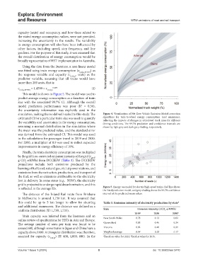
This model is shown in Figure 5. The model was used to
predict average energy consumption as a function of train
size with the associated 99.7% CI. Although the overall
model prediction performance was poor (R = 0.30),
2
the uncertainty information was explicitly used in the
simulation, making the model well-suited to this study. The Figure 4. Visualization of Net Zero Vehicle Emission Model correction
estimated CI for a particular train size was used to quantify algorithms for tank-to-wheel energy consumption (and emissions),
the variability and uncertainty in the energy consumption, reflecting the impacts of changes in articulated truck mass for different
driving conditions. The 99.7% prediction and confidence intervals are
assuming a normal distribution in the simulation where shown by light grey and dark grey shading, respectively.
the mean was the predicted value, and the standard error
was derived from the estimated CI. This model was used
in the calculations for passenger travel in 2019 and 2030.
For 2050, a multiplier of 0.9 was used to reflect expected
improvements in energy efficiency of 10%.
Finally, the train electricity consumption was multiplied
by the grid-loss-corrected emission intensity of the grid (ε ,
grid
g CO -e/kWh) from DCCEEW (Table 3). The DCCEEW
2
projections include both emissions produced by the
burning of fuel (coal, natural gas, etc.) at power stations, and
emissions from the extraction, production, and transport of
the fuel, as well as emissions attributable to the electricity
lost in delivery. In some states (e.g., NSW), the electricity
grid is projected to undergo rapid decarbonization, and this
is reflected in the average EIs. Figure 5. Energy use model for electric high-speed trains. Red line shows
the fitted prediction model, and grey shading shows the 99.7% confidence
The distance of the Inland Rail route from Brisbane interval of the predicted mean values.
to Melbourne is around 1,730 km. It was assumed that
this could be up to 5 km longer to allow for shunting Table 3. Emission intensity of electricity production by state 4
and additional maneuvers. The distance was defined as a
uniform distribution (U: 1,730, 1,735). State Emission intensity (t CO ‑e/MWh)
2
2019 a 2030 2050 b
Train capacity was inferred from the literature and an
online review of specifications for HSTs in Asia and Europe. New South Wales 0.78 0.13 0.02
The average number of seats per train was found to be Queensland 0.88 0.46 0.24
around 600, although some trains in Japan and China have a Victoria 0.92 0.40 0.39
capacity above 1000. A triangular distribution was, therefore, Weighted average 0.84 0.28 0.17
assumed for capacity (c (rail,p) ) (T: 400, 1,000, 600). In the a Based on value for 2022; fixed at value for 2035.
b

Volume 1 Issue 1 (2024) 8 doi: 10.36922/eer.3470