Page 74 - IJAMD-1-1

International Journal of AI
for Material and Design Machine learning for gripper state prediction

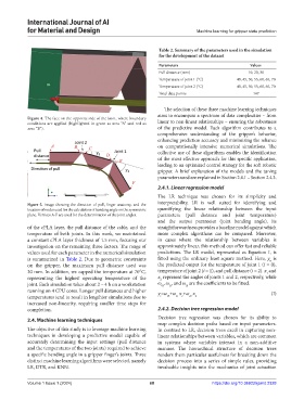
Table 2. Summary of the parameters used in the simulation
for the development of the dataset
Parameters Values
Pull distance (mm) 10, 20, 30
Temperature of joint 1 (°C) 40, 45, 50, 55, 60, 65, 70
Temperature of joint 2 (°C) 40, 45, 50, 55, 60, 65, 70
Total data points 147

The selection of these three machine learning techniques
aims to encompass a spectrum of data complexities – from
Figure 4. The face on the opposite side of the knot, where boundary
conditions are applied (highlighted in green as area “A” and red as linear to non-linear relationships – ensuring the robustness
area “B”). of the predictive model. Each algorithm contributes to a
comprehensive understanding of the gripper’s behavior,
enhancing prediction accuracy and minimizing the reliance
on computationally intensive numerical simulations. The
collective use of these algorithms enables the identification
of the most effective approach for this specific application,
leading to an optimized control strategy for the soft robotic
gripper. A brief explanation of the models and the tuning
parameters used are explained in Section 2.4.1 – Section 2.4.3.
2.4.1. Linear regression model
The LR technique was chosen for its simplicity and
interpretability. LR is well suited for identifying and
Figure 5. Image showing the direction of pull, finger anatomy, and the
location of nodes used for the calculation of bending angle on the symmetric quantifying the linear relationship between the input
plane. Vertices A-F are used for the determination of the joint angles. parameters (pull distance and joint temperature)
and the output parameter (joint bending angle). Its
of the cPLA layer, the pull distance of the cable, and the straightforwardness provides a baseline model against which
temperature of both joints. In this work, we maintained more complex algorithms can be compared. Moreover,
a constant cPLA layer thickness of 1.5 mm, focusing our in cases where the relationship between variables is
investigation on the remaining three factors. The range of approximately linear, this method can offer fast and reliable
values used for each parameter in the numerical simulation predictions. The LR model, represented as Equation I, is
is summarized in Table 2. Due to geometric constraints fitted using the ordinary least square method. Here, y is
n
on the gripper, the maximum pull distance used was the predicted output for the temperature of joint 1 (i = 0),
30 mm. In addition, we capped the temperature at 70°C, temperature of joint 2 (i = 1), and pull distance (i = 2). x and
1
representing the highest operating temperature of the x represent the angles of joints 1 and 2, respectively, while
2
joint. Each simulation takes about 2 – 4 h on a workstation ω , ω , and ω are the coefficients to be fitted.
0i
1i
2i
running on 4 CPU cores. Longer pull distances and higher y =ω +ω x +ω x (I)
temperatures tend to result in lengthier simulations due to i 0i 1i 1 2i 2
increased non-linearity, requiring smaller time steps for
completion. 2.4.2. Decision tree regression model
2.4. Machine learning techniques Decision tree regression was chosen for its ability to
map complex decision paths based on input parameters.
The objective of this study is to leverage machine learning In contrast to LR, decision trees excel in capturing non-
techniques in developing a predictive model capable of linear relationships between variables, which are common
accurately determining the input settings (pull distance in systems where variables interact in a non-additive
and the temperatures of the two joints) required to achieve manner. The hierarchical structure of decision trees
a specific bending angle in a gripper finger’s joints. Three renders them particular usefulness for breaking down the
distinct machine learning algorithms were selected, namely decision process into a series of simple rules, providing
LR, DTR, and KNN. invaluable insights into the mechanics of joint actuation

Volume 1 Issue 1 (2024) 68 https://doi.org/10.36922/ijamd.2328