Page 75 - IJAMD-1-1

International Journal of AI
for Material and Design Machine learning for gripper state prediction

and consequent bending behavior. The criterion for splits = 5 and n_repeats = 3, evaluated the performance
splitting used is the mean squared error, with the best-split of each machine learning algorithm, as described in
approach used by the splitter. Optimal hyperparameters Section 2.4, using mean absolute error (MAE) as the
were determined through a grid search method, resulting criterion to determine optimum hyperparameters. These
in a maximum depth of 9, minimum sample splits of 1, and data points were split into an 8:2 ratio for the training and
a minimum sample in the leaf node of 2. validation datasets in each iteration. The final model for
each algorithm was trained on the entire dataset with the
2.4.3. K-nearest neighboring regression model optimum hyperparameters. The accuracy of the best model

K-nearest neighbor regression was chosen for its from the three algorithms was tested against an additional
effectiveness in capturing intricate patterns in datasets five new untrained test conditions (providing 10 data
with complex interactions. KNN relies on the premise that points with the two joint angles), in which the predicted
similar input parameters yield similar output responses, output from the model was simulated, and the resultant
which is particularly relevant for our gripper model. In joint angle was compared against the input to verify the
this model, bending behavior was hypothesized to be performance of the model.
closely related to the specific configurations of stiffness
and pull distance. KNN can adaptively predict the bending 3. Results and discussion
angles by analyzing the “neighborhood” of data points 3.1. Analysis of the kinematics of the joint stiffness-
with similar features, providing a form of instance-based tunable gripper through numerical simulation
learning that is highly adaptable to new data. Optimum
hyperparameters, determined through a grid search The flexibility of the gripper to demonstrate various
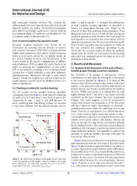
method, include two neighbors, a uniform weight for the combinations of joint angles by altering the temperatures
weight function, and the use of the Manhattan metric for at the joints is depicted in Figure 6. It is observed that
distance calculations. there are three different clusters of data points; each cluster
appears to be associated with a different pull distance of
2.5. Training procedure for machine learning 10 mm, 20 mm, and 30 mm, as indicated by the labels on
The 147 samples for the machine learning algorithm the plot. Within each cluster, it is noticed that the joint
training are depicted in Figure 6. Input features, consisting angles between joint 1 and joint 2 are almost inversely
of angles of joint 1 and joint 2, were trained against the correlated as the ratio between the joint temperature
temperature of joint 1, joint 2, and pull distance. To changes. This result suggests a kind of compensatory
avoid overfitting and underfitting of data, the repeated relationship between the temperatures of the two joints
k-Fold cross validator from the sklearn module, with n_ and their respective angles. Interestingly, we observed a
peculiar phenomenon within the mid-range of each data
cluster. Contrary to expectations of a uniform transition,
there exists a narrow region where data points overlap –
evidenced by the coalescence of red and dark red dots. This
pattern recurs across various pull distance clusters and
serves as an indicative sign of the non-linearity inherent
in the system’s behavior. This complexity and non-linearity
underscore the challenges of predicting system behavior
using traditional methods. Consequently, it reaffirms the
necessity of applying machine learning techniques for
forecasting in this context.
Figure 7 depicts the correlation between joints at varying
joint temperatures with one of its joints at the softest state.
Figure 7A shows the joint angle ratio of joint 1 to joint 2, γ /
1
γ , under varying joint temperatures at joint 2, while joint 1
2
is at its softest state (70°C). It is evident that the ratio of γ /γ 2
1
is higher when there is a significant temperature difference
between the two joints. Conversely, this ratio approaches
Figure 6. The distribution of samples by the angle of joint 1 and joint 1 when both joints are at the same temperature. Likewise,
2 and the kinematics of the gripper under the influence of varying
joint temperatures. The color scale represents the ratio of the joint 2 Figure 7B shows the joint angle ratio of joint 2 to joint 1,
temperature to the joint 1 temperature (T Joint 2 /T Joint 1 ). γ /γ , with different joint temperatures at joint 1 while joint
2
1
Volume 1 Issue 1 (2024) 69 https://doi.org/10.36922/ijamd.2328