Page 61 - IJAMD-1-2

International Journal of AI for
Materials and Design
AI-assisted ML monitoring in additive auxetics

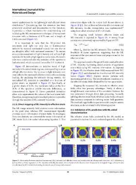
sensor applications for its lightweight and efficient stress conversion aligns with the output field dataset shown in
distribution. Considering that the structure has been Figure 1B [iii]. For calibration between effective strain and
46
extensively analyzed and documented in the literature, ML intensity, bicubic interpolation was implemented,
47
it provides a robust foundation for understanding and using four subset windows of 25 × 25 pixels.
validating the ML measurement technique. A honeycomb The mapping result between effective strain and
structure with a thickness of 0.75 mm and a length of ML intensity is depicted in Figure 5A. A strong linear
3 mm was used (Figure 4E). correlation is observed, represented by Equation VII:

It is important to note that the 3D-printed ML
specimens emit light not only due to luminescence (I ML =137 × ε equiv ) (VII)
induced by external mechanical stimuli but also due to where I denotes the ML intensity. This confirms the
ML
an afterglow effect with sustained emission. To ensure feasibility of linear regression, suggesting that the ML
45
an accurate assessment of light intensity and achieve high response of the specimen is linear and proportional to the
reproducibility with a high signal-to-noise ratio, the tensile effective strain.
tests were conducted after the emission of the specimens
had saturated, which occurred 2 min after UV treatment. This approach enables the quantification and calibration
of ML intensity, facilitating direct analysis of equivalent
Figure 4E demonstrates an intuitive trend of high strain fields using ML intensity information. As depicted
intensity in localized strain regions, corresponding to areas in Figure 5B, the effective strain field measured from DIC
of high effective strain. The increase in light intensity over (Figure 5B[i]) and obtained via transformed ML intensity
time reflects the increased effective strain with increasing values (Figure 5B[ii]) displays similar patterns with
loading. By analyzing the intensity during tension, the increasing global strain. The results indicate consistency in
normalized ML intensity is quantified as a function of the effective strain fields obtained by the two approaches.
global strain, as depicted in Figure 4F. Specifically, at
a global strain of 0.3%, the maximum values at the four Mapping the measured ML intensity to effective strain
ROIs of the specimen exhibit intensity differences, as fields offers two primary advantages. Firstly, it allows a
demonstrated in Figure S2. These quantified intensities straightforward examination of the correlation between the
allow us to approximate the values of the local strain field. two parameters through direct data processing. Secondly,
Therefore, recognizing local strain field patterns is possible utilizing effective strain fields, which are scalar fields, enhances
through the analysis of ML intensity variations. data accuracy compared to utilizing vector field quantities.
This method is applicable to specimens with complex auxetic
3.2.3. Direct mapping of ML intensity to effective strain structures, as demonstrated in the following section.
The ML image intensity field contains scalar information
at the pixel level, whereas DIC measurement typically 3.3. Validation of DL prediction with ML-aided
provides vector information of strain fields. To investigate characterization
these two datasets, we converted the vector information of The effective strain fields predicted by the DL model, as
DIC strain fields into scalar values using Equation 5. This presented in Section 3.1, were evaluated against the effective

A B

Figure 5. Relationship between mechanoluminescent (ML) intensity and effective strain and visualization in a honeycomb structure. (A) Calibration is
derived from a linear regression of ML intensity with effective strain. (B) Comparison of effective strain measured by (i) digital image correlation and
(ii) calculated by ML transformed during the tensile test of honeycomb structure.

Volume 1 Issue 2 (2024) 55 doi: 10.36922/ijamd.3539