Page 48 - IJAMD-1-3

International Journal of AI for
Materials and Design
Metal AM porosity prediction using ML

a layer is critical in the manufacturing process since a slight separately on the “low” and “high” datasets were trained.
variance in the porosity at this level could affect the overall Then, the models evaluate their performance on the unseen
quality of the built product. held-out test dataset. Figure 9 illustrates the absolute error
and RMSE scores of the two models. The black dotted line
As shown in Figure 7, the significant split in the
distribution (x-axis) observed in Figure 3 is absent once represents the identity line, and the red line denotes the
we split the dataset. Hence, there is no clear distinction line of best fit.
between the two distributions once we separate the dataset Figure 10A shows the performance of the XT regressor
into “low” and “high” subsets. Therefore, predicting on the “low” porosity dataset. The model achieves a low
the porosity level should be more challenging than RMSE score of 0.0367, echoed in the absolute n error
classification. plot, as the best-fit line fairly aligns with the identity line.
Likewise, the model has also achieved a relatively low RMSE
3. Results and discussion score of 0.108 on the “high” porosity dataset (Figure 10B).

3.1. Regression However, the best-fit line has a slightly different slope
compared to the “low” dataset result, showcasing a slightly
All the regression models were evaluated using the RMSE weaker performance.
separately on the “low” and the “high” porosity training
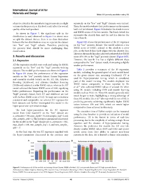
datasets. The models’ performances are shown in Figure 8. Table 2 provides a summary of the 10 regression
In Figure 8A shows the performance of the regression models, including the general speed of each model based
models on the “low” porosity dataset. Linear Regression on the given dataset size, assuming GridSearch CV is
and ensemble models (which are RF, XT, GB, Adaptive used for hyperparameter tuning, which is considered
Boosting [AdaBoost], and eXtreme Gradient Boosting part of the model training. The models displayed low
[XGBoost]) attained similar RMSE values, whereas the XT RMSE values comparable to those reported by Ho
57
model achieved the lowest RMSE score of 0.04, signifying et al. who achieved RMSE values of around 5% when
better performance. Regarding the performance on the using DL models including CNN and transfer learning
“high” porosity dataset, both XT and AdaBoost are tied models such as VGG‑16. These DL models generally take
much longer to train, highlighting a strong advantage of
with the best RMSE score of 0.12. To keep our evaluations 21
consistent and comparable, we selected XT regressor for these ML models. Liu et al. also reported the use of ML in
both datasets and further investigated this model in the predicting porosity, achieving significantly higher RMSE
values between 10% and 26%, which are much higher
hyper-parameter optimization stage.
compared to those achieved in this study.
The best hyper-parameters for the XT regressor The execution time of Python scripts can be measured
model from Grid SearchCV on the “low” dataset are: using the time function to provide an indication of model
n_estimators = 700, max_depth = 76, min samples_leaf = 2, and performance. LR is the fastest in terms of real-time
min_samples_split = 2. The best hyper-parameters discovered processing due to the simplicity of solving a single linear
for the model on the “high” dataset are: n_estimators = 841, equation and the absence of hyperparameter tuning.
max_depth = 138, min_samples_leaf = 2, and min_samples_ However, the preference for models like XT over LR,
split = 3.
despite similar RMSE values (0.05 and 0.04) and slower
As the final step, the two XT regressors supplied with speed, stems from their ability to capture non-linear
the hyper-parameters discovered in the previous step patterns in the data. LR is limited to linear relationships,

A B

Figure 8. Performance of all the models on training dataset (lower RMSE is better): (A) Low‑porosity layers and (B) high‑porosity layers.
Abbreviations: AdaB: Adaptive Boosting; DT: Decision Tree; GB: Gradient Boosting; k-NN: k-Nearest Neighbors; LR: Linear Regression; RF: Random
Forest; RMSE: Root‑mean‑square error; SVR: Support Vector Regression; XGB: eXtreme Gradient Boosting; XT: Extremely Randomized Trees.

Volume 1 Issue 3 (2024) 42 doi: 10.36922/ijamd.4812