Page 65 - IJAMD-2-1

International Journal of AI for
Materials and Design
Fatigue life prediction via contrastive learning

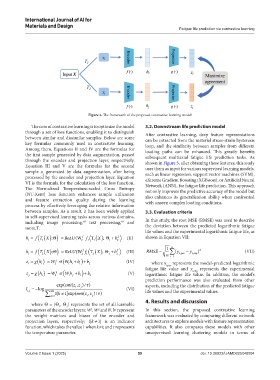
Figure 4. The framework of the proposed contrastive learning model

The core of contrastive learning is to optimize the model 3.2. Downstream life prediction model
through a set of loss functions, enabling it to distinguish After contrastive learning, deep feature representations
between similar and dissimilar samples. Below are some can be extracted from the material stress-strain hysteresis
key formulas commonly used in contrastive learning. loop, and the similarity between samples from different
Among them, Equations II and IV are the formulas for loading paths can be enhanced. This greatly benefits
the first sample generated by data augmentation, passed subsequent multiaxial fatigue life prediction tasks. As
through the encoder and projection layer, respectively. shown in Figure 5, after obtaining these features, this study
Equation III and V are the formulas for the second uses them as input for various supervised learning models,
sample x generated by data augmentation, after being such as linear regression, support vector machines (SVM),
j
processed by the encoder and projection layer. Equation eXtreme Gradient Boosting (XGBoost), or Artificial Neural
VI is the formula for the calculation of the loss function. Network (ANN), for fatigue life prediction. This approach
The Normalized Temperature-scaled Cross Entropy not only improves the predictive accuracy of the model but
(NT-Xent) loss function enhances sample utilization also enhances its generalization ability when confronted
and feature extraction quality during the learning with unseen complex loading conditions.
process by effectively leveraging the relative information
between samples. As a result, it has been widely applied 3.3. Evaluation criteria
in self-supervised learning tasks across various domains,
including image processing, text processing, and In this study, the root MSE (RMSE) was used to describe
66
67
more.T. the deviation between the predicted logarithmic fatigue
life values and the experimental logarithmic fatigue life, as
f
f TX ; ReLU( W f f T X ; b (II) shown in Equation VII:
i
h 1 2 1 1 1 2
1 n
f
f TX ; ReLU( W f f T X ; b (III) RMSE y ( y ) 2 (VII)
i
h 2 2 1 2 1 2 ipre, iexp,
n i1
b
g
z W Wh b 2 (IV) where y i,pre represents the model-predicted logarithmic
g h
2
1
1
i
i
i

g h
b
g
z W Wh b 2 (V) fatigue life value and y i,exp represents the experimental
logarithmic fatigue life value. In addition, the model’s
1
2
j
i
1
j
prediction performance was also evaluated from other
(,
exp( smiz z )/ ) aspects, including the distribution of the predicted fatigue
l log i j (VI)
ij,
2 k1 1 k [ 1 ]exp( smi zz )/ ) life values and the experimental values.
N
(,
j
i
4. Results and discussion
where Θ = {Θ , Θ } represents the set of all learnable
1
2
parameters of the encoder layers; W, W and b, b represent In this section, the proposed contrastive learning
f
g
f
g
the weight matrices and biases of the encoder and framework was evaluated by comparing different network
1]
projection layers, respectively; 1[k ≠ is an indicator architectures to explore models with feature representation
function, which takes the value 1 when k≠i; and τ represents capabilities. It also compares these models with other
the temperature parameter. unsupervised learning clustering models in terms of
Volume 2 Issue 1 (2025) 59 doi: 10.36922/IJAMD025040004