Page 57 - IJB-6-2

Zolfagharian, et al.
density ρ appropriate sensitivities for a particular properties [25,27] , and inserting Equation (13) in
e
element can calculated as follows [27,29,30] : Equation (12), the sensitivity could be determined:
 obj ,e  1 (  e T  K u T  u  u e  u u K K u e )  Obj ,e 1 p 1 − T , (14)
T
) 
e
1
 e 2V  e e e e ∂  e e e e  e  e = − 2V e (E − 2 E p e uK u
0,ee
e
(5)
Applying the system equation Ku = f to a single 2.2 Sensitivity filtering
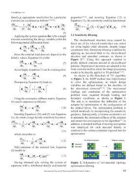
element considering the design variable yields the The checkerboard structure issue caused by
following partial differential form: direct use of the selected sensitivities was sorted
 e + K u K e u =  f e ( 6) out using higher order elements, despite longer
e  e  e e  e calculation time. Sensitivity filtering is utilized by
Since the external load does not depend on the applying an increased limit to the checkerboard
density values, Equation (6) yields: structure and smoother contours, as shown in
Figure 2 . Using this approach resulted in
[26]
∂K ∂u
e u + K e = 0 (7) poorly defined contours instead of checkerboard
∂ρ e e e ∂ρ e patterns. Digital pixel structures are adapted to the
Accordingly, Equation (7) can be rearranged to: finite element mesh to allow the image processing
.
results to be directly applied to TO problem
[31,32]
K
K e ∂ u e =− ∂ ∂ρ e u (8) in Figure 3, the SIMP method was implemented
As shown in the flowchart of TO algorithm
e
∂ρ
e
e
Transposing Equation (8) leads to: to solve the optimization, in which design
 ∂ u  T  ∂ K  T variables are defined based on the densities of
 K e ∂ρ   =− ∂ρ e u e   (9) the discretized elements [33-35] . The mechanical
e



loadings and constraints of the optimization
e
e
problem were modeled through loading and
Using the symmetric stiffness matrix, Equation boundary conditions, as shown in Figure l.
(9) can be expressed as follows: The aim is to maximize the deflection of the
actuator by optimization of the configuration of
∂u T e K =−� u T ∂K e (10) the printed layers. The optimization problem is
∂ρ e e e ∂ρ e solved iteratively by incorporating the sensitivity
Inserting Equations (10) and (9) into Equation guidance. Subsequently, a volume constraint is set
(5), the strain energy density sensitivity becomes: to minimize the structural stiffness of the actuator
[36]
∂Π 1 ∂K ∂K ∂K and ensure the convergence of the algorithm . In
obj e, = (−u T e u + u T ∂ e u − u T e u ) addition, a standard method of moving asymptotes
∂ρ e 2 V e e ∂ρ e e e ∂ ρ e e e ∂ρ e e was employed for each material density to
(11) conform to the volume constraint imposed into the
which simplifies to: optimization.
Π 1 ∂K
Obje, =− u T e u . (12)
∂ρ e 2 V e e ∂ρ e e
Differentiation of the material law, Equation
(2) results in:

∂K e = K ( E − ) p−1 (13)
Epρ
∂ρ e 0, e 2 1 e
Having obtained u by solving the system of Figure 2. Schematics of two-material topology
e
equations with a distributed density and material optimization filtering.

International Journal of Bioprinting (2020)–Volume 6, Issue 2 53