Page 14 - IJOCTA-15-3

A. Kaveh, M. Vahedi, M. Gandomkar / IJOCTA, Vol.15, No.3, pp.379-395 (2025)
instance, at a sampling time of h = 0.005, the generated. Therefore, to stabilize this section, we
fractional-order system reaches a stable equilib- consider the variable q = 0.995.
rium point. On the other hand, for a sampling Considering that the controlled system is an
time of h = 0.05, the conventional system be- order-fractional system, the desired sliding sur-
comes unstable from the sampling time, as illus- face must also have an order-fractional form. We
trated in Figure 6. define the sliding surface such that S → 0 cor-
responds to x 2 → 0; therefore, according to the
fractional-order system in Equation (18), we de-
fine the slip surface in the form of Equation (19)
29
:

q 2 −1
S = D t x 2 (t) (19)
According to Equation (18), if x 2 → 0, then
x 1 → 0 and x 3 → 0, which transforms the prob-
lem into a regulation problem.

3.2. Control input design
Next, the control input u is defined as follows: 4–6

u = u eq + u N (20)
as u eq is the equivalent control component, which
keeps the states on the sliding surface. u N is the
switching component that directs the states to the
sliding surface. u N is primarily responsible for
stabilizing the system and is designed using the
Lyapunov stability criterion.

∂S
˙
˙
S(x) = · X(t)
∂X
∂S
= [f(t, x) + B(t, x)(u eq + u N )]
∂X
∂S
= [f(t, x) + B(t, x)(u eq + u N )]
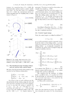
Figure 6. The chaotic state trajectories of the ∂X
fractional order brushless direct current system ∂S ∂S
without a control signal with h = 0.005 and h = 0.05 = [f(t, x) + B(t, x)u eq ] + B(t, x)u N
∂X ∂X
∂S
= B(t, x)u N
3.1. The fractional-order brushless direct ∂X
current system with control input (21)
if we assume that ∂S B(t, x) = I , where I is the
∂X
We know that the fractional-order equation is rep- identity matrix, then we have S(x) = u N , which
˙
resented by the following relationship:
satisfies this condition sufficiently.
The condition for the existence of sliding

˙
q 1
 D x 1 = −x 1 + x 2 x 3 mode ( condition S i S i < 0 ) is given by S ̸= 0.
0 t
q 2 (18) In the following, we will describe two important
t
0 D x 2 = −x 2 − x 1 x 3 + µx 3

q 3
 D x 3 = −σ(x 3 − x 2 ) and commonly used cases in this article for the
0 t
discontinuous control section:
According to the no-load conditions and the (a) Relay with constant gain:
characteristics of this section, using the trial and
error method or drawing the bifurcation diagram, (
−α i Sign(S i (x)), S i (x) ̸= 0, α i > 0
it can be seen that the system is unstable for
u i N =
0 < q 1 = q 2 = q 3 = q < 0.6 and ∨ q > 1.1 0, S i (x) = 0
conditions and when 0.6 < q < 0.98 converges (22)
to one of the two equilibrium points of E 2 ∨ E 3 , where the sign function is meant. It is observed
and for 0.99 < q < 1.1, chaotic behavior is that choosing this option for the discontinuous
386