Page 18 - IJOCTA-15-3

A. Kaveh, M. Vahedi, M. Gandomkar / IJOCTA, Vol.15, No.3, pp.379-395 (2025)
that the proposed FO-SMC strategy outperforms surface of the proposed method. A comparison
conventional SMC, offering superior stability, ro- is made with normal sliding mode control, which
bustness, and adaptability in controlling chaotic is naturally applied to the normal derivative sys-
FO-BLDC systems. tem, to determine the advantages of the proposed
To evaluate the performance of the controllers method.
used in this paper, we use the following error met-
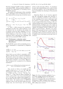
rics, which are the average sum of absolute errors: Observing Figure 12, it becomes apparent
that the conventional sliding mode strategy re-
 Z T
1 sults in a significant overshoot in the current i d
E x = |) dt

 (|e x 1 | + |e x 2 | + |e x 3
T
 at the beginning of the period, which may cause
T 0
1 Z T the system to become saturated. Additionally,
E x−dot = (|e x 1 −dot | + |e x 2 −dot | + |e x 3 −dot |) dt


T it can be observed that the current i q in the con-
T 0
(35) ventional sliding mode strategy exhibits irregular,
= x 1d − x 1 , e x 1 −dot = ˙x 1d − ˙x 1 , and frequency-based oscillations over time, which re-
where e x 1
T = T s .t f . duces the system’s overall performance quality. In
In Table 1, which presents the quantitative contrast, the proposed method results in a com-
comparison of these two control methods, it can pletely smooth behavior. Therefore, the perfor-
be observed that by calculating the average sum mance of the proposed method is more desirable.
of absolute errors, the state regulation errors are Furthermore, the Omega plot indicates that the
somewhat close to each other, but there is a sig- superiority of the proposed method is evident, as
nificant difference in the rate of change of state it exhibits better convergence speed and fewer os-
regulation errors, indicating the advantage and cillations.
value of the proposed FO-SMC method.
4.2. Performance evaluation under
parameter uncertainties and external
disturbances
The FO-BLDC system with uncertainties and ex-
ternal disturbances is represented by Equation
(36):


q 1
0 D x 1 = −x 1 + x 2 x 3
t
q 2
0 D x 2 = −x 2 − x 1 x 3 + γx 3 + u(t) + ∆g(x 1 , x 2 , x 3 ) + d(t)
t
0 D x 3 = −σ(x 3 − x 2 )
 q 3
t
(36)
where ∆g (x 1 , x 2 , x 3 ) refers to parameter uncer-
tainties, and d(t) refers to external disturbances.
We aimed to observe the behavior and resistance
of the system in response to these changes by ap-
plying them as inputs to the system. Moreover,
these sentences are considered as the following
equations: 10

∆g(x 1 , x 2 , x 3 ) = 10.75 sin (10x 1 (t) cos (3x 2 (t) cos(πx 3 (t))
d(t) = 5.25 cos(2x 2 (t)) + 8.5 sin(3t)
(37)
Now, similar to before, we consider the pa-
rameter vector as (µ, γ, σ) = (1, 20, 5.46), the
homogeneous orders of the system as q 1 = q 2 =
q 3 = 0.995, and T sim = 6 sec. The time con-
stant is h = 0.005, and the initial conditions as
Figure 12. State trajectories regulation of i d , i q ,
(x 1 (0), x 2 (0), x 3 (0)) = (5, 5, 5). A switching gain
and Omega variables in fractional-order BLDC
of k = 5 is used, and relation (32) is designed us-
system using FO-SMC signal in the presence of
ing the sign function based on the sliding mode
parameter uncertainties and external disturbances
control input. Its implementation in MATLAB Abbreviations: BLDC, brushless direct control;
software is used to plot the state paths, the state FO-SMC, fractional-order sliding mode controllers;
change rate, the control input, and the sliding SMC, sliding mode controller
390