Page 150 - IJOCTA-15-3

E.M. Shaban / IJOCTA, Vol.15, No.3, pp.517-534 (2025)

" #
F 1,k F 2,k F 3,k (13)
F k = |{z} |{z} |{z}
(n+m+δ−1)×3 (n+m+δ−1)×(n−2) (n+m+δ−1)×(m+δ−2)
(n+m+δ−1)×(n+m+δ−1)
" # T
−b 1,k −b 1,k −b 1,k 0 0 . . . 0 0 1 0 . . . 0 0
(12)
g k = | {z } | {z } | {z }
3 n−2 m+δ−2
" #
0 −1 0 0 0 . . . 0 0 0 0 . . . 0 0
h = | {z } | {z } | {z }
3 n−2 m+δ−2
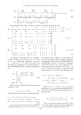
The submatrices F 1,k , F 2,k , and F 3,k are defined as follows in Equation (13).

As depicted in Equation (13), the submatri- the submatrix F 2,k vanishes, and the third col-
ces F 2,k and F 3,k exist if and only if n > 2 and umn in the submatrix F 1,k becomes zero-valued.
m + δ > 2, respectively. Therefore, in case of Consequently, this results in the NMSS/SDP-PI+
n = 2 and m + δ = 2, there is no plus, and representation without a derivative component,
the definition in Equation (12) is downgraded to as the third column vector of the submatrix F 1,k ,
the NMSS/SDP-PID form as follows in Equation associated with the derivative state, ∆e k−1 , is
(14). zero. 17 Under this condition, the states defined
in Equations (9-11) are reduced to Equation (17).
 
1 − (a 1,k + a 2,k ) a 2,k
F k = 0 − (a 1,k + a 2,k ) a 2,k ,


e k = − a 1,k e k−1 − b 1,k u k−1 − . . .
0 − (a 1,k + a 2,k + 1) a 2,k
 
−b 1,k (14) − b m−1,k u k−(m−1) − b m,k u k−m
g k = −b 1,k , (17)


z k =z k−1 − a 1,k e k−1 − b 1,k u k−1 − . . .
−b 1,k
− b m−1,k u
and h = 0 −1 0 k−(m−1) − b m,k u k−m
Here, the state feedback vector is as presented
in Equation (15), Thus, for n = 1 and m + δ > 2, the set
of Equation (17) represents the NMSS/SDP-PI+
T
form using the following state feedback vector in
x k = z k e k ∆e k (15)
Equation (18).
for which the states are given as in Equation (16).
T
e k = − (a 1,k + a 2,k ) e k−1 + a 2,k ∆e k−1 − b 1,k u k−1 z k e k u k−1 u k−2 ...,
x k = (18)
z k = z k−1 − (a 1,k + a 2,k ) e k−1 + a 2,k ∆e k−1 − b 1,k u k−1 u k−(m+δ−3) u k−(m+δ−2)
∆e k = − (a 1,k + a 2,k + 1) e k−1 + a 2,k ∆e k−1 − b 1,k u k−1
(16) The state transition square matrix F k (order
Also, in the case of the discrete-time SDP-TF m + δ), the input vector g , and the observation
k
model with unity order, i.e. n = 1, and m+δ > 2, vector h are now defined as Equation (19).
522