Page 151 - IJOCTA-15-3

Proportional integral derivative plus control for nonlinear discrete-time state-dependent parameter. . .

 
 
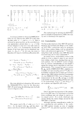
1 −a 1,k −b 2,k −b 3,k . . . −b m+δ−2,k −b m+δ−1,k 1 −a 1,k 0 −b 2,k −b 3,k . . . −b m+δ−2,k −b m+δ−1,k
 0 −a 1,k 
0 −a 1,k −b 2,k −b 3,k . . . −b m+δ−2,k −b m+δ−1,k  0 −b 2,k −b 3,k . . . −b m+δ−2,k −b m+δ−1,k 

0 0 0 0 . . . 0 0   0 −a 1,k 1 2 −b 2,k −b 3,k . . . −b m+δ−2,k −b m+δ−1,k 


2
2
2
2
2


0 0 1 0 . . . 0 0   0 0 0 0 0 . . . 0 0 




 . . . . . . . . . . . . . .  F k = 0 0 0 1 0 . . . 0 0 
F k = 

. . . . . . .   . . . . . . 
 .


. . . . . . . . . .
  . . . . . . . . 
0 0 0 0 0 0
 . .   
 . . 
0 0 0 0 0 1 0  0 0 0 0 0 . 0 0 
0 0 0 0 0 . . . 1 0

n = 1

n = 1 ↔
↔ m + δ > 2
m + δ > 2
h i T
T g k = −b 1,k −b 1,k −b 1,k 1 0 . . . 0 0
g k = −b 1,k −b 1,k 1 0 . . . 0 0 2 2 2

h = 0 −1 0 0 0 . . . 0 0
h = 0 −1 0 0 . . . 0 0
(22)
(19)
The methodology for deriving the SDP-PID+
and its variants is summarized in Table 1 for clar-
It is always possible to derive the NMSS/SDP- ity and to disentangle the equations.
PID+ for the discrete-time SDP-TF model with
the first order, n = 1, and m + δ > 2. This is
3.2. Controllability
achieved by assuming that, as the controlled pro-
cess approaches a steady state, i.e. e k → 0, the The linear-like structure of the SDP-TF model in
second difference of the error state also tends to Equation (4) facilitates the design of the nonlin-
2
zero, i.e., ∆ e k → 0. Consequently, the first dif- ear SDP-PID+ control law using the strategies
ference of the error state can be considered con- of the linear system design, such as suboptimal
∼
stant, i.e., ∆e k = c. 13 In this case, the states in LQ or pole assignment approaches. 10–15 However,
Equation (17) may be rewritten as Equation (20). using these basic methods, some SDP-TF model
structures may not be fully controllable. 38
In control theory, controllability refers to the
ability to drive a system’s state to any desired
e k = −a 1,k e k−1 − b 1,k u k−1 − . . . state within a finite time, starting from any ini-
− b m−1,k u k−(m−1) − b m,k u k−m tial condition. For the SDP-TF model in Equa-
tion (4), discrete controllability at each sample k
z k = z k−1 − a 1,k e k−1 − b 1,k u k−1 − . . .
means the system can be controlled at each sam-
− b m−1,k u k−(m−1) − b m,k u k−m pling instance. This, necessarily, leads to a system
∆e k + ∆e k−1 F k , g , and h of NMSS/SDP-PID+, which is con-
k
∆e k = 38,39
2 trollable over each sampling period. The con-
− (a 1,k + 1) e k−1 − b 1,k u k−1 − . . . trollability conditions can be stated as: 39 Given a
−b m−1,k u k−(m−1) − b m,k u k−m + ∆e k−1 discrete-time SISO system described by Equation
= (4), the NMSS/SDP-PID+ form in Equation (7),
2
(20) characterized by the pair [F k and g ], is locally
k
controllable over each sampling period if and only
if, the polynomials A χ k , z −1 and B χ k , z −1
The state definition in Equation (20) restores are co-prime, and Equation (23) is met.
the NMSS/SDP-PID+ form for the first-order
m
SDP-TF model using the following state feedback X −(j+δ−1)
b j+δ−1 {χ k } z ̸= 0 (23)
vector in Equation (21).
j=1
Due to the time-varying nature of the parame-
ters in the SDP case, it is important to note that
these conditions may not always be met in ev-
T
z k e k ∆e k u k−1 u k−2 ...,
x k = (21) ery sample period. As a result, challenges may
u k−(m+δ−3) u k−(m+δ−2) emerge during the control design process for the
SDP-PID+ controller.
Although deriving comprehensive results for
The square matrix F k of order m + δ + 1 the controllability and stability of the nonlin-
(∀ n = 1), the input vector g , and the obser- ear SDP system remains an area of ongoing
k
vation vector h are defined as Equation(22). research, 38,39 the practical approach described
523