Page 155 - IJOCTA-15-3

Proportional integral derivative plus control for nonlinear discrete-time state-dependent parameter. . .
Rockwool blocks insulate the tank’s exterior to
minimize heat loss and reduce power consump-
tion.
A motorized three-way valve and a PT100
temperature sensor are integrated into this ther-
mal process and connected to a data acquisition
unit (LabJack UE9) interfaced with a LabVIEW™
program. The valve’s opening is normalized from
0 (fully closed) to 100 (fully open) to regulate the
flow rate of the hot oil, functioning as an actua-
tor. The PT100 provides temperature feedback
for the control system. A LabVIEW™ module
was developed to manage the hardware compo-
nents (three-way valve and PT100 sensor) and
apply the selected controller. Additional hard-
ware/software interfacing details can be found in
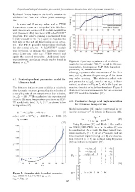
Hamed et al. 40 Figure 6. Open loop experiment and simulation
results for the estimated SDP-TF model for bitumen
temperature. Abbreviations: SDP, State-dependent
parameter; TF, transfer function
where y k represents the temperature of the bitu-
men, and u k denotes the percentage of the three-
way valve opening. The state-dependent out-
4.1. State-dependent parameter model for
put parameter a 1 (χ k ), denoted as a 1,k , is time-
bitumen tank
variant, as shown in Figure 5, while the input pa-
The bitumen tank’s process exhibits a relatively rameter, denoted as b 3 , is time-invariant. Figure 6
slow dynamic response, prompting the selection of illustrates the simulation results for the estimated
a sampling rate of one sample every four minutes, SDP-TF model in Equation (37).
i.e., ∆t = 240 . 40 The analysis of the experimental
data for Bitumen temperature produces an SDP-
13
TF model with triad {1, 1, 3} , as shown below 4.2. Controller design and implementation
for Bitumen temperature
in Equation (37)
Model in Equation (37) can be represented by us-
y k = −a 1 (χ k ) y k−1 + b 3 u k−3 (i) ing the operator z −1 as follows in Equation (38).
a 1 (χ k ) = 0.1 × 10 −5 y 2 k−3 − 0.00135 y k−3 − 0.995 (ii) b 3 z −3
b 3 = 0.063 y k = −1 u k (38)
1 + a 1 (χ k+1 ) z
(37)
Using Equation (38) and Table 1, the nonlin-
ear NMSS/SDP-PID+ form in Equation (7) can
be constructed. As a result, the time-variant tran-
sition matrix F k (5 × 5) at the k th sample, and the
time-invariant input vector g (5 × 1) and observa-
tion vector h (1 × 5) are defined using Equation
(22) as follows in Equation (39).

 
1 −a 1 (y k−3 ) 0 0 −b 3
0 −a 1 (y k−3 ) 0 0 −b 3 
−a 1 (y k−3 ) − 1 1
 
 −b 3 
F k = 0 0  ,
2 2
 2 
0 0 0 0 0
 
0 0 0 1 0 (39)
 
0
0
 
 
Figure 5. Estimated state-dependent parameter, g = 0 , h = 0 1 0 0 0
 
 
1
a 1,k , versus its state variable y k−3 , i.e.  
a 1,k = f (y k−3 ) 0
527