Page 152 - IJOCTA-15-3

E.M. Shaban / IJOCTA, Vol.15, No.3, pp.517-534 (2025)
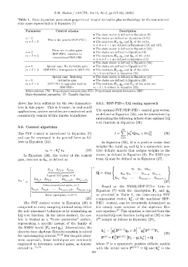
Table 1. State-dependent parameters-proportional integral derivative plus methodology for the non-minimal
state space representation in Equation (7)

Parameter Control scheme Description
• The state vector is defined in Equation (8)
n ≥ 2 • The states are defined at Equations (9-11)
This is the general SDP-PID+
m + δ > 2 • The matrices, F k , g , and h, of the order,
k
n + m + δ − 1 are defined in Equations (12) and (13).
• The state vector is defined in Equation (15)
There are no plus gains
n = 2 • The states are defined in Equation (16)
SDP-PID+ switches to
m + δ = 2 • The matrices, F k , g , and h k , of the order
k
conventional SDP-PID
n + m + δ − 1 are defined in Equation (14)
• The state vector is defined in Equation (18)
n = 1 Special case: No derivative gain • The states are defined in Equation (17)
m + δ > 2 SDP-PID+ downgrades to SDP-PI+ • The matrices, F k , g , and h, of the order
k
m + δ are defined in Equation (19)
Special case: Restoring • The state vector is defined in Equation (21)
n = 1 derivative gain • The states are defined in Equation (20)
m + δ > 2 SDP-PI+ is upgraded back to • The matrices, F k , g , and F k , of the order are
k
SDP-PID+ m + δ + 1 defined in Equation (22)
Abbreviations: PI+: Proportional integral plus; PID: Proportional integral derivative; SDP:
State-dependent parameter; TF: Transfer function.
above has been sufficient for the two demonstra- 3.3.1. SDP-PID+/LQ tuning approach
tors in this paper. This is because, in real-world
The optimal SVF/SDP-PID+ control gain vector,
applications, system variables are constrained and
as defined in Equation (25), can be determined by
consistently remain within known boundaries.
minimizing the following infinite-time optimal LQ
cost function in Equation (26).
3.3. Control algorithm
∞
T
The SVF control is introduced in Equation (5) J = X x Q x k + R u 2 k (26)
k
and can be expressed in its general form as fol- k=0
lows in Equation (24). In Equation (26), R is a positive scalar that
weights the input u k and Q is a symmetric pos-
+
u k = −k x k (24) itive definite matrix that assigns weights to the
k
In Equation (24), the vector of the control states, as defined in Equation (8). For SISO sys-
gain, denoted as k k , is defined as tems, Q may be defined as in Equation (27).

 
  T
k I,k k P 1 ,k k D,k ,  q z q e 1 q ∆e, 
 Q = diag · · ·
| {z }
 q e 2 q e 3 q e n−2 q e n−1,
Typical PID gains, n≤2
   
  . . .
q u 1 q u 2 q u m+δ−3 q u m+δ−2
+  k P 2 ,k k P 3 ,k . . . k P n−2 ,k , k P n−1 ,k , 
K K (27)
=  | {z } 
 
Extra proportional gains, n>2
  Based on the NMSS/SDP-PID+ form in
k
 
k
 u 1 ,k k u 2 ,k . . . k u m+δ−3 ,k , k u m+δ−2 ,  Equation (7) with the description F k and g
| {z } k
Extra input gains, m+δ≥2 as provided in Table 1, the time-varying SVF
+
(25) compensator vector, k , of the nonlinear SDP-
k
The SVF control vector in Equation (25) is PID+ control, can be recursively determined as
computed at every sampling interval using either the steady state solution of the algebraic Ric-
the pole placement technique or by minimizing an cati equation. 37 This equation is derived from the
LQ cost function. In the latter method, the sys- standard LQ cost function in Equation (26) at the
tem is treated as a “frozen parameter” system, k th sample as follows in Equation (28),
representing a specific instant of the family of
the NMSS model [F k and g ]. Alternatively, the h i −1
k + T (i+1) T (i+1)
discrete-time algebraic Riccatti equation is solved k = g P g k + R g P F k (28)
k
k
k
for each sampling interval. 33,36 For the pole place- (i) T (i+1) +
P = F P F k − g k k + Q
ment approach, linear techniques are commonly k k
employed to determine control gains, as demon- where P is a symmetric positive definite matrix
strated in . 11,12 with the initial value P (i+1) = Q and k + is the
k
524