Page 130 - MI-2-3

Microbes & Immunity Statistical modeling of COVID-19 trends

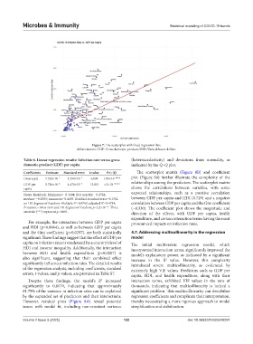
Figure 7. The scatterplot with fitted regression line
Abbreviations: GDP: Gross domestic product; USD: United States dollars.

Table 6. Linear regression results: Infection rate versus gross (heteroscedasticity) and deviations from normality, as
domestic product (GDP) per capita indicated by the Q–Q plot.
Coefficients Estimate Standard error t‑value Pr(>|t|) The scatterplot matrix (Figure 8B) and coefficient
−8
(Intercept) 7.523×10 −2 1.254×10 −2 6.001 1.05×10 *** plot (Figure S8) further illustrate the complexity of the
GDP per 5.736×10 −6 4.470×10 −7 12.831 <2×10 *** relationships among the predictors. The scatterplot matrix
−16
capita shows the correlations between variables, with some
expected relationships, such as a positive correlation
Notes: Residuals: Minimum=−0.3404; first quartile: −0.0784;
median=−0.0503; maximum=0.4639. Residual standard error=0.1352 between GDP per capita and HDI (0.729) and a negative
2
on 181 degrees of freedom. Multiple R =0.4763; adjusted R =0.4734; correlation between GDP per capita and the Gini coefficient
2
F-statistic=164.6 on 1 and 181 degrees of freedom; p=2.2×10 . Three (−0.330). The coefficient plot shows the magnitude and
−16
asterisks (***) represent p<0.001. direction of the effects, with GDP per capita, health
expenditure, and certain interaction terms having the most
For example, the interaction between GDP per capita pronounced impacts on infection rates.
and HDI (p=0.0064), as well as between GDP per capita
and the Gini coefficient (p=0.0297), are both statistically 4.7. Addressing multicollinearity in the regression
significant. These findings suggest that the effect of GDP per model
capita on infection rates is moderated by a country’s level of The initial multivariate regression model, which
HDI and income inequality. Additionally, the interaction incorporated interaction terms, significantly improved the
between HDI and health expenditure (p=0.0007) is model’s explanatory power, as indicated by a significant
also significant, suggesting that their combined effect increase in the R value. However, this complexity
2
significantly influences infection rates. The detailed results introduced severe multicollinearity, as evidenced by
of the regression analysis, including coefficients, standard extremely high VIF values. Predictors such as GDP per
errors, t-values, and p-values, are provided in Table S7. capita, HDI, and health expenditure, along with their
2
Despite these findings, the model’s R increased interaction terms, exhibited VIF values in the tens of
significantly to 0.8179, indicating that approximately thousands, indicating that multicollinearity is indeed a
81.79% of the variance in infection rates can be explained significant problem. This multicollinearity can destabilize
by the expanded set of predictors and their interactions. regression coefficients and complicate their interpretation,
However, residual plots (Figure 8A) reveal potential thereby necessitating a more rigorous approach to model
issues with model fit, including non-constant variance simplification and stabilization.

Volume 2 Issue 3 (2025) 122 doi: 10.36922/MI025040007