Page 438 - IJB-10-3

International Journal of Bioprinting Different modeling of porous scaffolds

Quantum GX II), which allowed for the documentation of law, given in Equation II. 32-34 To facilitate the calculation,
the external structure and the calculation of porosity. The the ratio of height H to H was set to be equal to e. The
1
2
CT scan parameters were set to 90 kV for voltage, 80 μA time difference t (t = t - t ) was recorded for the fall of the
1
0
for current, and 14 min for scanning duration. The top horizontal plane.
of the porous scaffolds was imaged using a JEM-2100F lg H − lg H
scanning electron microscope, and DM software was used k = µ hA × 1 2 (II)
to analyze structural features, including pore size and ρ gta lg e
strut dimensions.
The parameters used in the formula are selected and
2.3. Mechanical performance testing shown in Table 2.
According to the mechanical testing standard, ISO
13314, for porous and cellular metallic materials, 29-31 Using the computational fluid dynamics software
compression and tensile tests were conducted at room ANSYS 16.0 Workbench with the Fluent module, a fluid
temperature using an electronic universal testing simulation analysis was conducted on individual scaffold
machine (Suns, Shenzhen, China). At least three samples units, as illustrated in Figure 3B. The entrance flow velocity
were compressed for each structural sample. The was set to 0.01 m/s to investigate the structural factors
compression strain rate was set at 0.5 mm/min until the affecting permeability, with an outlet pressure of 0 Pa.
samples became fully dense or fractured. The fracture The wall was assumed to be non-slip, and the minimum
morphology of the scaffolds was recorded using a unit size was set to 0.01 mm to analyze the effect of the
camera. Stress–strain curves were plotted; yield strength, modeling strategy on the permeability from a microscopic
ultimate strength, elastic modulus, and other mechanical point of view.
properties were calculated; and the data were expressed
as mean ± standard deviation (SD). 3. Results and discussion
2.4. Permeability performance testing and 3.1. Macro- and microscopic characteristics
simulation of scaffolds of scaffolds
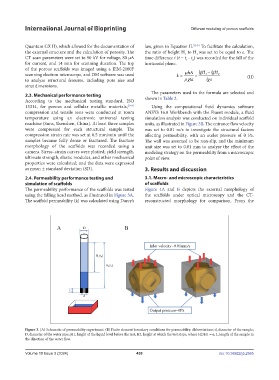
The permeability performance of the scaffolds was tested Figure 4A and B depicts the external morphology of
using the falling head method, as illustrated in Figure 3A. the scaffolds under optical microscopy and the CT-
The scaffold permeability (k) was calculated using Darcy’s reconstructed morphology for comparison. From the

Figure 3. (A) Schematic of permeability experiment. (B) Finite element boundary conditions for permeability. Abbreviations: d, diameter of the sample;
D, diameter of the water pipe; H1, height of the liquid level before the test; H2, height at which the test stops, where H2/H1 = e; L, length of the sample in
the direction of the water flow.

Volume 10 Issue 3 (2024) 430 doi: 10.36922/ijb.2565